Western Blot Quantification Software
Measure Western blot band intensity from original images, subtract local background, normalize to a matched loading control and export the results to Excel.
Practice with built-in examples without signing in. Register for free figure tools and an eligible full-feature trial of up to one month, subject to account and device history. After online verification, use your authorized features offline on this computer for 30 days.
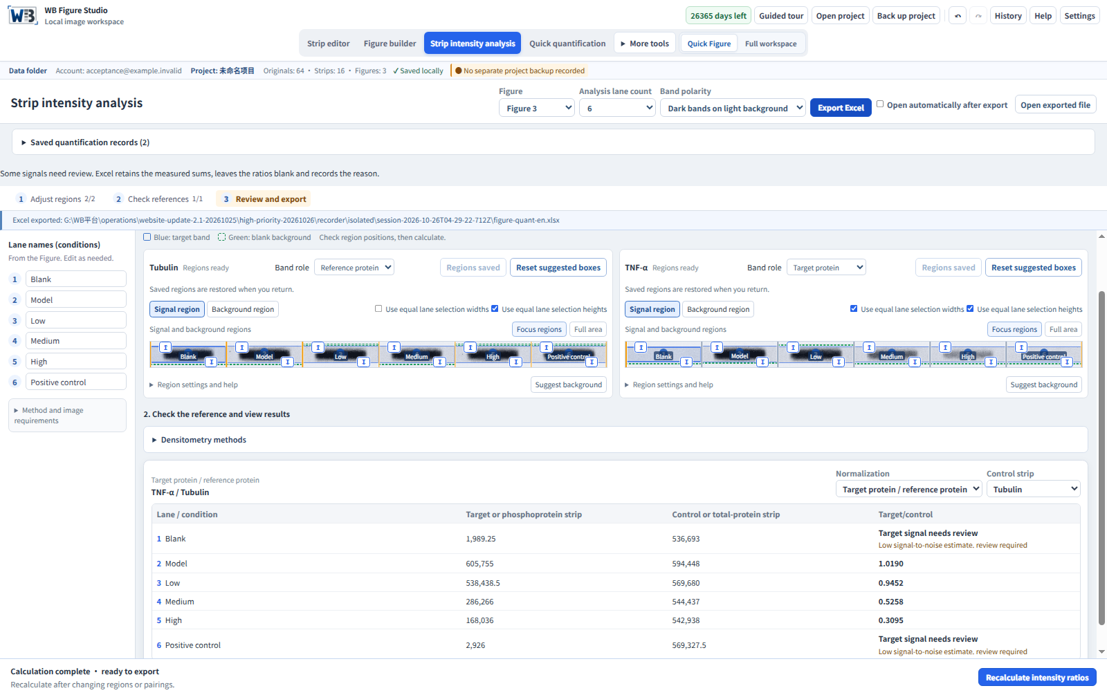
Trace each value to its original image and region
Consistent, adjustable regions
Lock region widths and heights while positioning each lane vertically.
Background-corrected densitometry
Review a separate, non-overlapping local-background region for each lane and correct original-pixel measurements.
Two normalization modes
Pair targets with a same-membrane control, or phosphoproteins with the corresponding total-protein bands. Review and adjust suggested matches.
Export results to Excel
Export integrated densities, normalized ratios, sample names and region coordinates for further analysis.
Archived build 1.1.40 walkthrough
Archived build40 quantification walkthrough
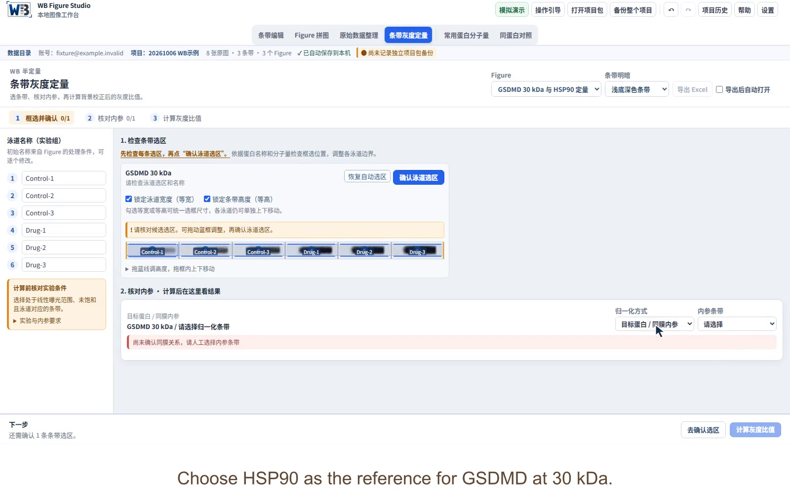
Confirm each lane region
Include the band and some local background. Match GSDMD and HSP90 to the same samples, then confirm both sets of regions.
Correct the background
In this archived build40 example, the app estimated background inside each region and sums the corrected pixel contributions. For Control-1, the corrected GSDMD integrated density is 196,661.28. Read the 2.0 method, which requires separate background regions.
Normalize to the reference
Divide each target intensity by its matching reference intensity. Control-1: 196,661.28 / 570,339.498 = 0.344814.
Export and review
Save the sample names, integrated densities, ratios and region coordinates in Excel. Open the practice workbook to inspect the result columns.
Follow the step-by-step instructions or watch the quantification tutorial.
From selected regions to usable results
Explore the Excel workbook from the build 2.1.3 demonstration above: measurements, ratios and review flags, with Calculation notes, Provenance and Measurements sheets. The data are simulated.
Archived practice data (1.1.x)
These archived practice results use native-roi-v2 from build 1.1.40. They are preserved to explain that workbook and are not 2.0 native-local-bg-v3 results. New calculations require separate background review.
| Sample | GSDMD 30 kDa ID | HSP90 ID | Target / reference |
|---|---|---|---|
| Control-1 | 196,661.28 | 570,339.498 | 0.344814 |
| Control-2 | 347,773.334 | 595,700.301 | 0.583806 |
| Control-3 | 453,455.721 | 569,879.948 | 0.795704 |
| Drug-1 | 560,005.848 | 554,410.766 | 1.010092 |
| Drug-2 | 601,098.838 | 540,119.46 | 1.112900 |
| Drug-3 | 655,234.915 | 519,953.806 | 1.260179 |
Displayed values are rounded for reading. Calculations use the preserved full-precision values.
View the two source pieces from one membrane
One membrane, cut into two pieces
The six samples share one membrane. After cutting along the dashed line, upper piece 1-1 is used for HSP90 at 90 kDa and lower piece 1-2 for GSDMD at 53/30 kDa. Lane order remains the same in both pieces.
Each piece has its own companion set. Keep both sets in one folder, import them together, then review each set separately.
Get started with this feature
Check the originals and exposure
Select a figure containing the target and reference strips. Check sample correspondence, band polarity, and that both target and reference signals fall within their validated linear detection ranges.
Match the loading control and lanes
Use target protein / same-membrane loading control, or phosphoprotein / corresponding total-protein band. Match the same samples and lane order, and check membrane identity and source grouping. Review suggested pairings; explicit roles and reference choices are retained.
Adjust and save each lane region
Switch between signal and background regions, then adjust the blue signal and green background boxes. Select nearby band-free background that does not overlap the signal. Review target and reference regions, then choose Save regions.
Calculate and review ratios
Review each sample’s target intensity, denominator intensity and ratio. After changing regions or pairings, review and calculate again.
Export the results and measurement record
Export Excel and review sample names, target and reference intensities, ratios and region records. Undefined ratios remain blank with a reason; do not treat them as zero. Keep the project and complete originals. Provenance records source checksums, bit depth and algorithm.
From normalized ratios to fold change
For this calculation example, choose the arithmetic mean of Control-1, Control-2 and Control-3 ratios as the baseline. These are synthetic practice lanes, not evidence of independent biological replicates.
Control baseline = (0.344814 + 0.583806 + 0.795704) / 3 ≈ 0.574775
Fold change = sample target/reference ratio / control baseline
| Sample | Exported ratio | Fold change |
|---|---|---|
| Control-1 | 0.344814 | 0.600 |
| Control-2 | 0.583806 | 1.016 |
| Control-3 | 0.795704 | 1.384 |
| Drug-1 | 1.010092 | 1.757 |
| Drug-2 | 1.112900 | 1.936 |
| Drug-3 | 1.260179 | 2.192 |
For Drug-1, 1.010092 / 0.574775 ≈ 1.757. The control group mean is 1 after this scaling, although individual control lanes differ.
The software exports target/reference ratios. Calculate fold change separately in your analysis worksheet. This step is not an automatic software output or a significance test. Select the baseline and treatment of biological and technical replicates according to your experimental design.
Review and save signal and local background regions
- In the quantification workspace, review strip roles and target/reference pairing. Use lossless instrument-exported PNG or TIFF images with 8/16-bit grayscale or RGB data. Multipage TIFFs are imported by page; select the appropriate measurement source. JPEG images may be used for layout, not quantification.
- The app suggests lanes and background. Batch suggestions preserve existing manual regions. Nearby original-image areas can supply new background suggestions. Switch between signal and background regions in each strip card. Move the blue signal box, green background box and their edges to cover the complete signal and nearby band-free background without overlap.
- Review each signal and background region, then check the denominator and lane correspondence. Calculate intensity ratios and export Excel. Save regions after manual changes to retain them when switching. Review and recalculate after changing regions or pairing.
Method and result explanations
Algorithm: native-local-bg-v3. Each original image pixel is counted once by its center. Screen rendering, display adjustments and rotation-interpolated intensities are not used. B is the mean of the separate background region, N is the number of original signal pixels, and I is pixel intensity.
Dark bands on light background
S = N × B − ΣILight bands on dark background
S = ΣI − N × BNegative results are retained. Negative per-pixel contributions are not clipped to zero. Endpoint pixels no longer block normalized output. Invalid denominators and unmeasurable inputs retain their reasons instead of producing Infinity or invented zeros. SNR below 3 is a noise-review threshold, not a certified limit of detection.
Existing records keep their original algorithm and values. Recalculation in the current version requires rechecking the separate background regions. Older videos, workbooks and build40 values below are not expected results for the new algorithm.
Normalization and interpretation
Sample ratio = target ID / same-membrane control ID
Phosphorylation mode calculates phosphoprotein ID / corresponding total-protein band ID. Here, total protein means the total form of the corresponding protein, rather than total-lane protein staining.
For fold change, divide sample ratios by a specified control baseline in your subsequent analysis. Identify biological and technical replicates and select statistical methods for the experimental design. Interpret changes alongside originals, saturation checks, exposure and reference stability.
Taylor et al. (2013), A Defined Methodology for Reliable Quantification of Western Blot Data
Version and calculation verification
Build 1.1.40: the same example recalculated
The same two 8-bit practice originals, crop coordinates and six lane regions were recalculated with native-roi-v2. That historical version preserves source precision and fractional bilinear samples. The old version rounded interpolated samples to 8-bit integers. All 12 integrated densities change slightly, so neither old video nor build40 values are expected outputs for the 2.0 algorithm.
| Sample | GSDMD | HSP90 | Recorded ratio | Build 40 ratio |
|---|---|---|---|---|
| Control-1 | 196,661.28 | 570,339.498 | 0.347402 | 0.344814 |
| Control-2 | 347,773.334 | 595,700.301 | 0.578580 | 0.583806 |
| Control-3 | 453,455.721 | 569,879.948 | 0.798574 | 0.795704 |
| Drug-1 | 560,005.848 | 554,410.766 | 1.010837 | 1.010092 |
| Drug-2 | 601,098.838 | 540,119.46 | 1.116641 | 1.112900 |
| Drug-3 | 655,234.915 | 519,953.806 | 1.256137 | 1.260179 |
These differences describe only this fixed example and do not establish results for other experiments or clinical use. The pack contains original SHA-256 checksums, crop and lane coordinates, the algorithm identifier and full-precision results. The original videos, workbook and verification pack remain unchanged.
Export target and control intensities together with normalized ratios, without transcribing results by hand.
| Sample | GSDMD 30 kDa | HSP90 | GSDMD / HSP90 |
|---|---|---|---|
| Control-1 | 197,930 | 569,743 | 0.3474 |
| Control-2 | 345,052 | 596,377 | 0.5786 |
| Control-3 | 454,863 | 569,594 | 0.7986 |
| Drug-1 | 559,450 | 553,452 | 1.0108 |
| Drug-2 | 603,472 | 540,435 | 1.1166 |
| Drug-3 | 653,915 | 520,576 | 1.2561 |
Control-1: 197,930 / 569,743 = 0.3474
This ratio compares target and reference signals in that sample. Fold change requires an additional division by a defined control baseline.
The pack contains two complete practice originals, ROI coordinates, sampled pixels and expected results. Twelve integrated densities and six ratios were checked with native build 1.1.24 and an independent script. The included instructions explain how to recalculate them. This example does not replace validation of your experiment’s linear range or loading control.
Frequently asked questions
How does the app subtract background?
B is the mean of a separately selected local-background region. Dark-band signal is N×B−ΣI. Light-band signal reverses this subtraction. Negative values are retained. Original pixels are counted once by their centers, independent of display adjustments.
How large should each region be?
Include the complete band while excluding adjacent lanes and unrelated signal. Choose a separate nearby, band-free background region without overlap. Apply a consistent selection strategy throughout the comparison.
Is HSP90 always a suitable loading control?
The example uses HSP90. For your experiment, validate that the control remains stable under the treatment conditions and lies within the linear detection range. This example uses the upper and lower pieces of one membrane. Match target and control to the same samples and check lane order.
How do I normalize a Western blot and calculate fold change?
The exported ratio is target integrated density divided by denominator integrated density. To express fold change, divide each sample ratio by a defined control baseline and document that additional analysis.
Can I directly compare different blots or saturated images?
Check saturation in the acquisition software and validate the experimental linear range. Saturation loses intensity information. Comparisons across blots require an appropriate experimental design, shared calibration and explicit reporting. A ratio alone does not remove exposure or batch effects.
Does the app calculate statistical significance?
2.0 adds quick analysis and biological-replicate summaries. Confirm independent samples, matching references and groups before reviewing individual points, summaries and applicable statistical suggestions. The app does not infer biological replicates from file counts.